Abstract
This project is a project on the topic on creating a stylized ocean environment in Unreal Engine 5. It consist of multiple areas of shader works including waves, water effects, WPO animation shaders, postprocessing effects, and multiple other shaders, all designed for underwater scene. Additonally, this project utilizes UE5’s Niagara particle system and its Neighbour grid3D to improve performance for simulating the movement of fish schools using the boids algorithm. Using the custom shaders and particle systems, I built an ocean environment, showcased from 2 different perspectives.
Preface
In this article, I will briefly go through the following techniques I’ve experimented with, the issues I’ve encountered, and their remedies separated into several stages in chronological order.
The area of coverage is larger than I initially expected. With that being said, it’s possible that I have made some mistakes and misunderstanding, in which case, please feel free to correct my understanding (´・ω・`).
You can also visit my repository here at fishies
Implementation and Stages
Part 1: Waves - Sine Waves, Gerstner Waves, Scrolling waves
Waves
Initially, this project was meant to only be focused on this section, making a simple ocean waves simulation where I try a few techniques on implementing wave shaders.
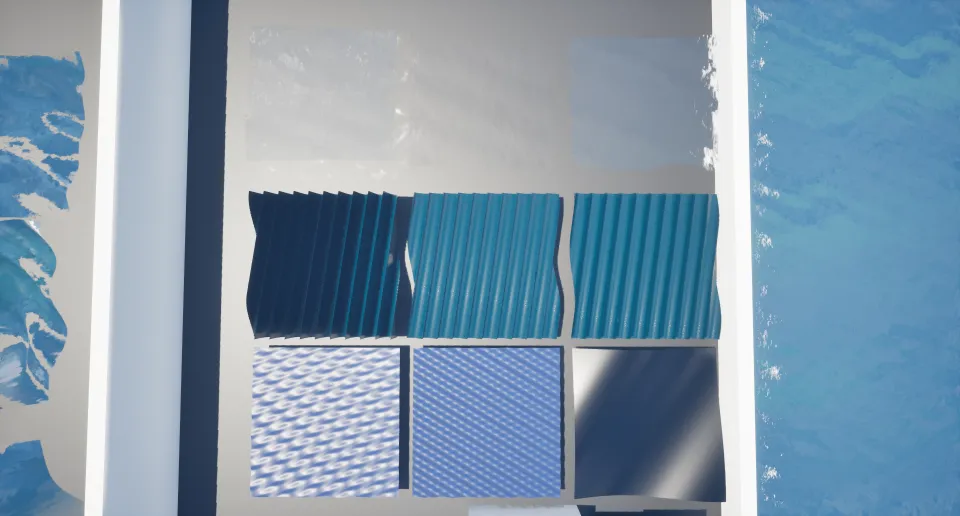
figure 01: Waves testing room
The idea of animating ocean-wave in general is to offset the vertices of the ocean-wave plane in a specific direction using a wave function. From here, we can use wave superposition by adding multiple waves with different amplitudes, wavelength, speed, etc.. together to create a more interesting shape. For this part, I’ve tried 2 different implementations.
Sine Waves
The first implementation I’ve tried my hands on is using sine waves where I offset the plane’s vertices in z direction only. This is probably the simplest method that uses World Position Offset for simulating waves.
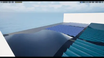
figure 02: Sine waves
Gerstner Waves
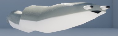
The second method here I tried and decided to use is gerstner waves, this method creates a more realistic waves with sharper peaks and wider trough. In contrary to the sine wave implementation, this wave offset moves the waves vertex in all xyz direction.
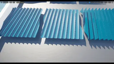
figure 03: Gerstner waves
Comparing the two waves
One of the benefits of using Gerstner waves is that, waves here creates wider trough than the sine waves.
However, this does not come without a drawback. When the steepness value gets too high $(>1)$ the wave will curl upon itself. (There are modified versions of sine wave that gives wider trough too but I didn’t use that.)
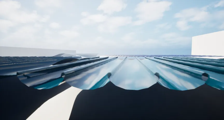
figure 04: Gerstner waves curling on itself
For this implementation, I choose to continue with gerstner wave since it produces sharper peaks and also that I simply wanted to try it out.
Calculating wave normals
After the offset are calculated, I use cross product of the Binormal and Bitangent to calculate the normal vector where binormal and bitangent can be derived from the partial derivative of the x and y offset function. Luckily for my case, the literature from GPU Gems have already provided the complete form of the normal vector calculation which saved alot of time.
Extra effects - Scrolling wave normals
Scrolling textures: Now to improve the visuals I have added scrolling textures as additional normals to give the waves surface a more interesting look.
Fresnel: Afterwards, a Fresnel term is added to ensure the wave is more opaque (more reflection) when viewing at a near-grazing incedence.
Depth-Opacity: To make the object underwater look less visible when it is deeper, an opacity-based depth is also calculated using scene-depth (translucent-material ignored) - pixel-depth (translucent material tested) and scale it down by the desired depth factor. This gives a good impression of depth under water surface.
Refraction: For refraction, I just set it to water’s refraction index which is 1.33. Now we can combine these method and make a pretty nice waves/water shader.
figure 05: Sum of Gerstner waves with added effects
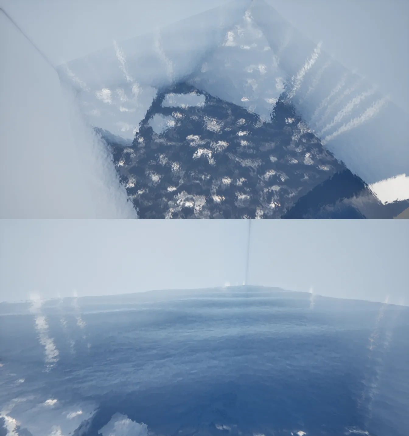
figure 06: Sum of Gerstner waves with view from above and grazing incidence
Issues, Remedies, and Considerations
Two sided waves
However, given that our wave is translucent. Since Unreal Engine uses Deferred rendering, the backface of the translucent waves are no longer culled giving a triangle looking visual artifacts.
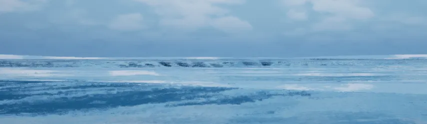
figure 07: Backface artifacts
To remedy this issue, I instead uses 2 water plane, made the material one-sided and disable the depth effect on the under-side of water where the under side does not use depth opacity check.
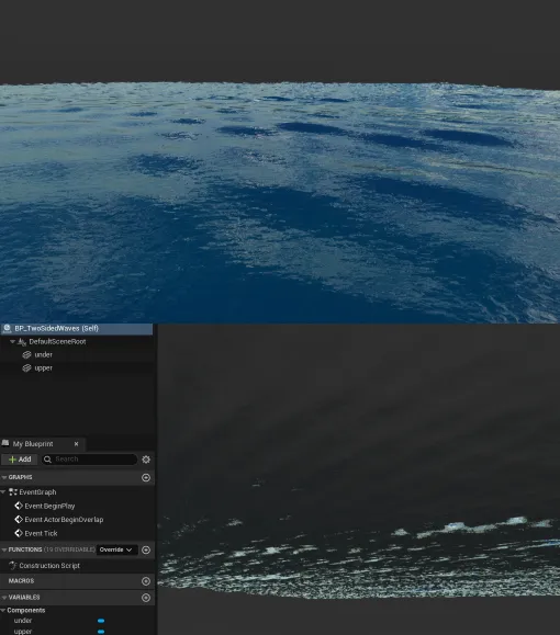
figure 08: Double plane wave
Mesh density and Nanite
The quality of the wave depends on the mesh density using this world position offset method. This means if this method were to be implement for a game, we should use higher vertex density mesh near the player or use a custom tesselation shader.
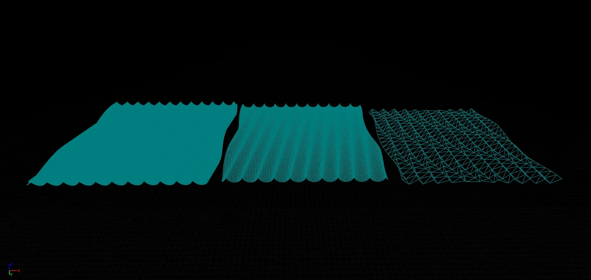
figure 09: Mesh density
I have to note that unreal engine’s nanite cannot be applied to this also since we uses the world position offset on the wave’s vertices and nanite would change the vertex position and density in a highly undesirable way.
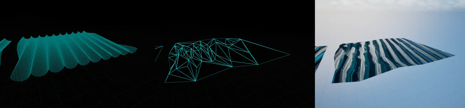
figure 10: Nanite Comparision
Blurring and Anti-Aliasing
When setting anti-aliasing to TSR, the blurring issue became very visible the higher the amount intensity the scrolling normal is. By lowering the scrolling normal intensity, the wave’s tiling effects became more visible. And when switching to FXAA, there are undesirable sharpness. I have yet to find a nice and balanced fix for this one.
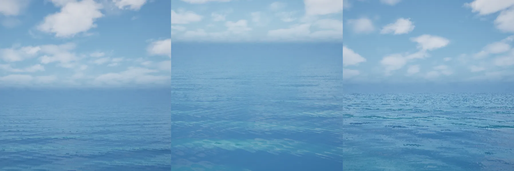
figure 11: High-intensity normal TSR, Low-intensity normal TSR, FXAA
Tiling and Alternatives
Both method of offsetting wave here introduces the undesirable effects of tiling. In this example it looks alright since it kind of resembles a calm ocean. However it cannot be denied that at certain angles the tiling became visible.
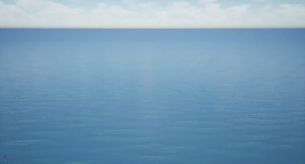
figure 12: Tiling
This means if we want a more realistic simulation, certain techniques suchas oceanographic spectra and FFT.
Final Implementation
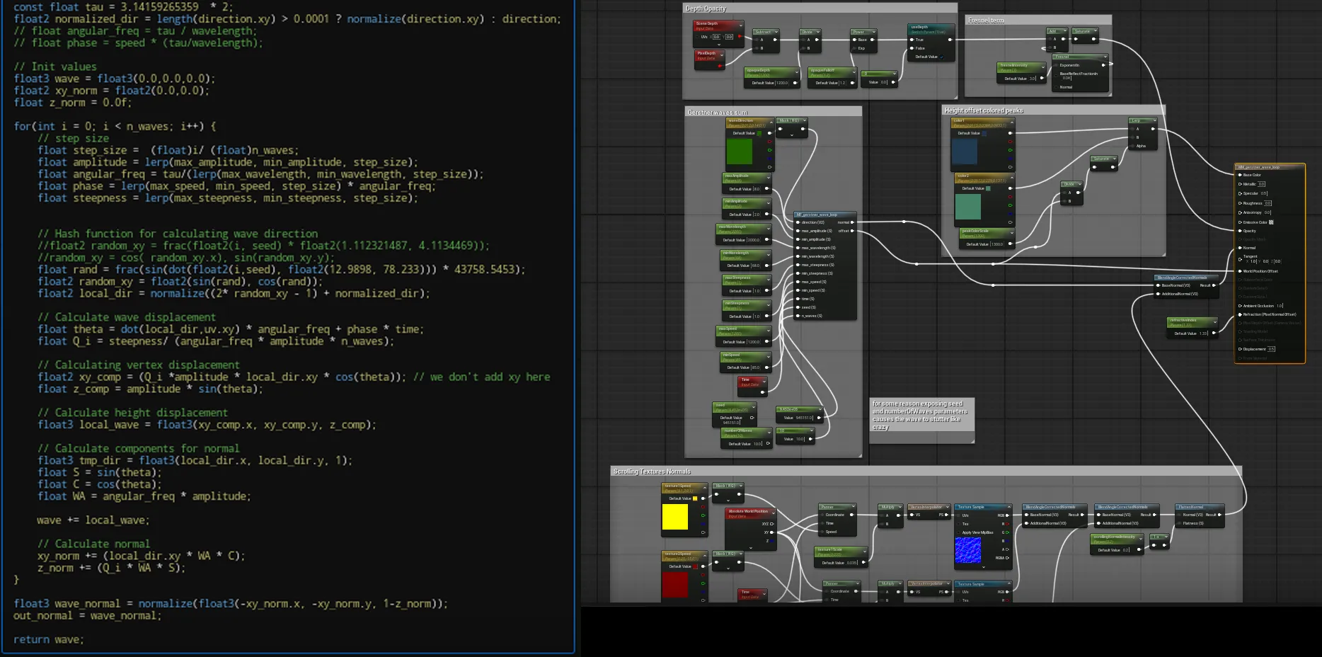
figure 13: Nodes and custom HLSL
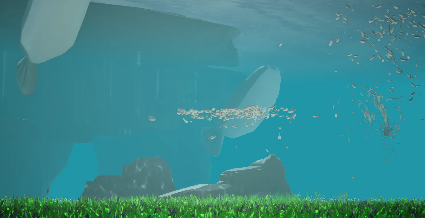
Part 2: Fishes - Boids
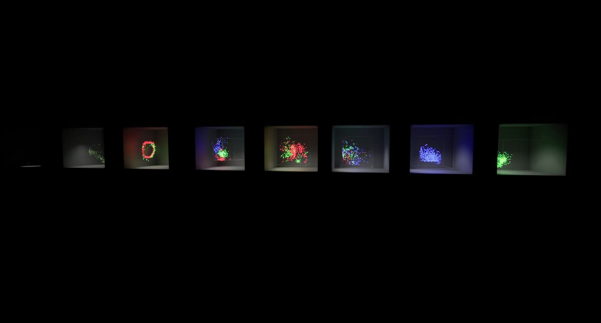
figure 14: Boids test room
Boids
Boids (bird-oid object) or a way to simulate flocking behaviour based on set of rules. There are three main factors when it comes to boids.
| Rules | Description |
|---|---|
| Separation | Each particle avoids each other |
| Alignment | Each particle steers in the direction of the flock |
| Cohesion | Each particle steers towards the center of the flock |
With these three rules, the particle will form an emerging behaviour
Neighbor Grid3D
To accelerate boids for real time use, I chose to use UE5’s built in Neighbor Grid3D inspired by this video from Ghislain Girardot (his visual debugger is super useful). Since I have never implemented this data structure myself, I will not go into details but here are the premises and use case of it.
The Neighbor Grid3D appears to be an implementation of a Bounded Spatial Hash Grid where the regions are divided into identical sized cells in xyz, direction. To figure out which cell the particle is in, you can applying a function based on the particle position which is stored inside a flatten 1d array. To make the flatten position works for dense grid, there are multiple techniques employed such as partial/prefix sum and so on…
In our use case, from there forward you can fetch the desired data of the neighbouring particle by iterating through the neighboring cells. (I’m glossing over a whole lot of things.)
This is particulary useful for things that utilizes local particle interaction rather than global interactions which makes it especially useful for fluid simulations, and in our case, boids.
Base Rules Force
In this implementation, the Neighbour Grid3D is used to fetch the cell of the current particle. Afterwards, I loop through the neighbouring cells index of the current cell and then iterates through each neighbouring particle in the cells.
After we get the neighboring particle positions, we calculate whether the particle is in the field of view using the dot product of the normalized current particle velocity and the direction of the current particle position to the neighbour.
If the neighboring particle is in the FOV, we can calculate the following forces.
// Calculate separation value
float separationRatio = 1 - clamp(length(directionParticleToNbrs) / inSeparationFalloff, 0, 1);

if (separationRatio > 1e-5)
{
    outSeparationForce -= separationRatio * directionParticleToNbrs; // -= since we are avoiding
    separationCount += 1.0;
}

// Calculate alignment value (flock direction)
float alignmentRatio = 1 - clamp(length(directionParticleToNbrs) / inAlignmentFalloff, 0, 1);

if (alignmentRatio > 1e-5)
{
    outAlignmentForce += alignmentRatio * normalize(nbrsVelocity);
    alignmentCount += 1.0;
}

// Calculate Cohesion value (flock center of mass)
float cohesionRatio = (1 - clamp(length(directionParticleToNbrs) / inCohesionFalloff, 0, 1)) ? 1 : 0;

if (cohesionRatio > 1e-5)
{
    outCohesionForce += nbrsPos * cohesionRatio;
    cohesionCount += 1.0;
}
We then take each ratio and divide them by the total count of particle, normalize the value, then scale it by a user defined factor.
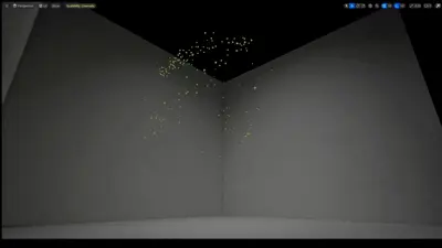
figure 15: 1 species boids
Extra force: Introducing several species, Predator-Prey force calculation
Boids species are distributed based on a user-defined curve.
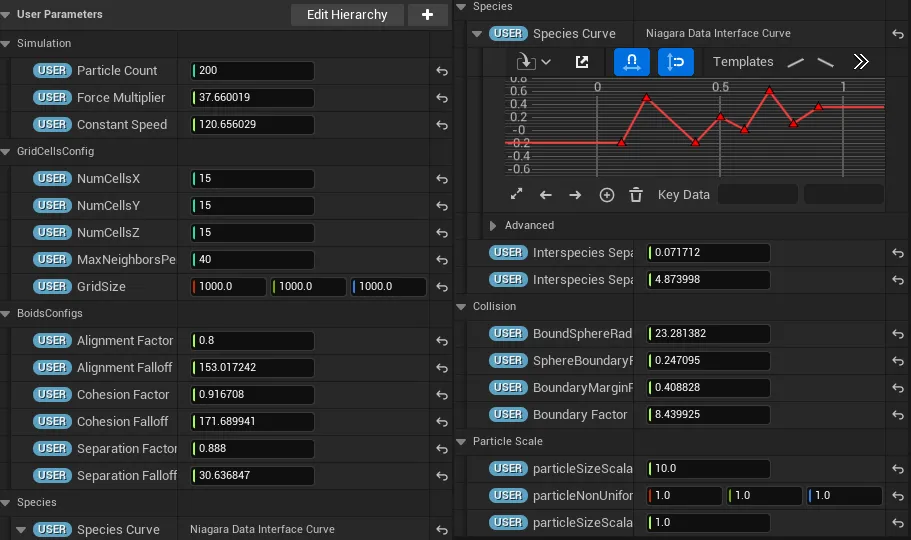
figure 16: User parameters
The rule in this implementation is simple and forces calculated very similary for intra species boids.
For particles that are in different species, they will avoid each other and will not align or cohese.
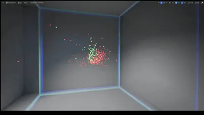
figure 17: 2 species boids
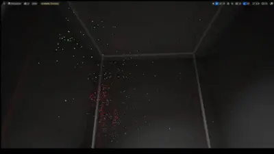
figure 18: 2 species boids
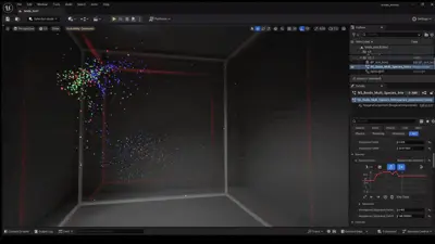
figure 19: 3 species boids
For Predator-Prey system, the prey will try to avoid predator and predator will try to follow prey. This, in my implementation however does not go well at all so I’ve decided to not use it.
Boundary Force: Setting boundaries
I use 3 ways initially to create boundary for keeping boids inside.
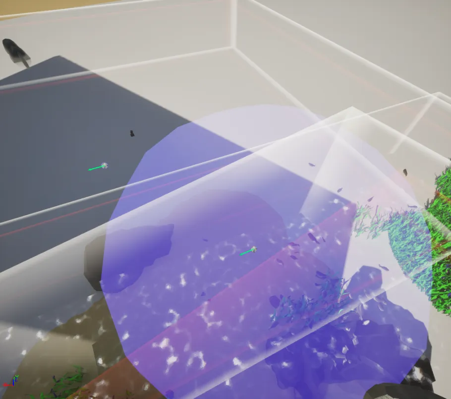
figure 20: 3 boundaries
The first method uses a box scaled by the scale of the particle system. If the particle goes out of bound, it will immediately reflects back in. This creates an undesirable effect of extremely sharp turn.
The second method also uses a box but then only apply forces when the particle goes out of bound for a smoother turn.
The third method creates a spherical region where the particles inside the region will not be affected by the force. However, when the particle leaves the region, it will apply a weak force to increase the tendency of particles to stay inside the region.
Applying Forces
The forces are applied into 2 stages
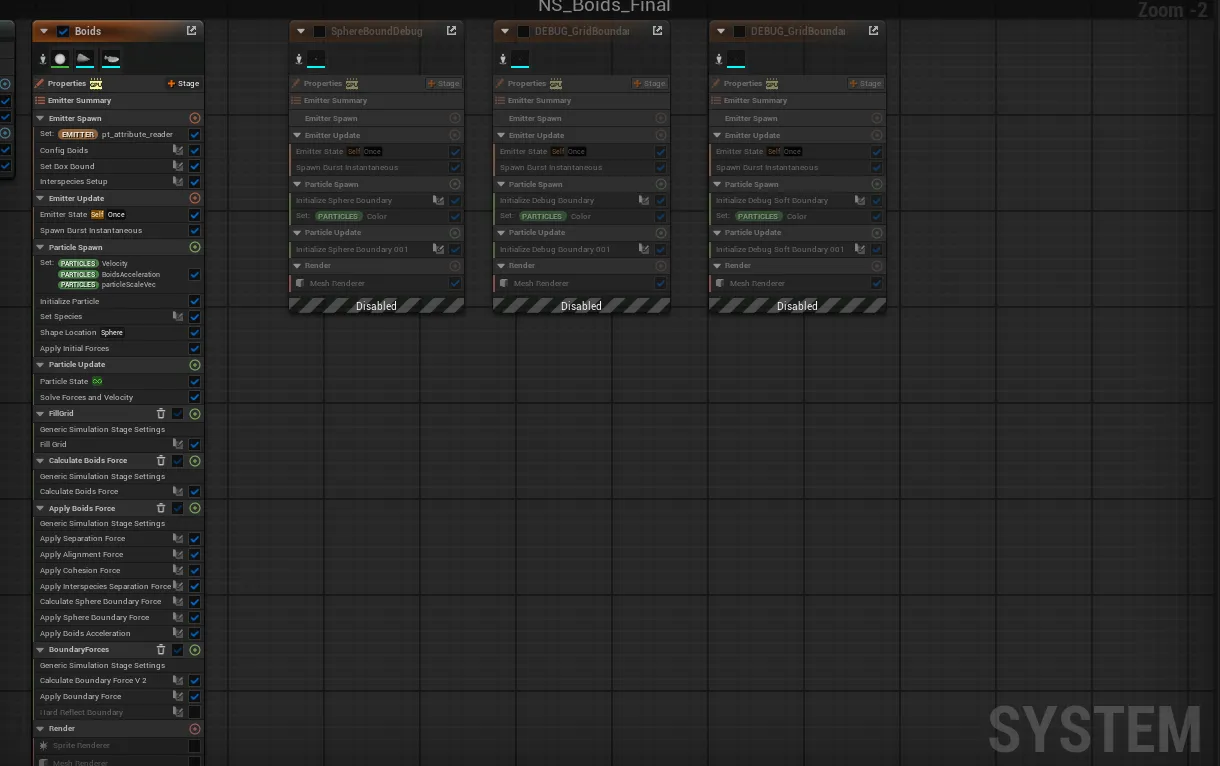
figure 21: Niagara system
Base Rule Force and Extra Force are added together with the velocity, scaled by delta time and a constant speed. (This somewhat gives a smoother movement)
Then in another pass the same is done with Boundary Force, this is to ensure the bounding force stays relatively strong.
WPO animation on fish vertex
The animation is done simply by using a simple wave function to offset the world positon
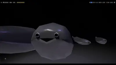
figure 22: Sacabambaspis
I should’ve vertex paint the face to mask the movement but it looks funnier this way (this mask doesn’t work in niagara system so the whole fish moves).
Final Implementation and Realization
This made me realize boids are so difficult to control and to make it work as desired.. The predator-prey system is difficulty to fine tune and would require quite more polishing to work properly. So for the final implementation I opted in to use the simple multi-species instead.
Part 3: Effects and Props - Caustics, Post-Processing, Foilage WPO animation, Setting up final scenes
Caustics
Since calculating caustics aren’t computationally cheap. The features of caustics are imitated with 2 textures.
The first texture is the base caustics, created using 2 4D smooth f1 voronois of the same position setup subtracing the one with lower scale, this create a smooth pattern resembling caustics (This technique is based on Deayan Studios).
To make it tileable, I put the UV positions through trig functions and added to the 4D voronoi function. The first texture is then baked using the add-on I wrote texture patisserie
Using the same setup, I created 3 other textures with minimal offset in xy direction to combine and create chromatic abberation effect.
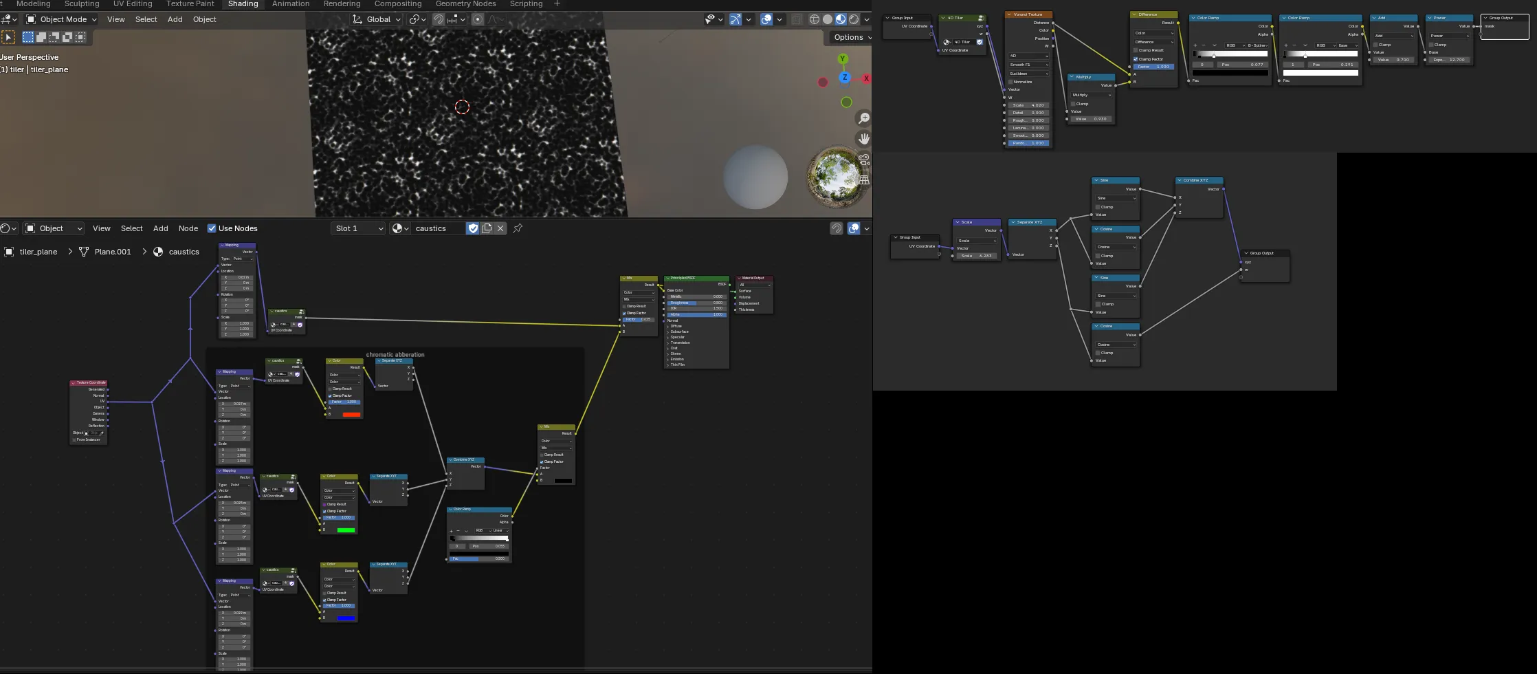
figure 23: Caustics Texture
The other texture is simply a scrolling wave texture which is added into the UV position of caustics to distort it.
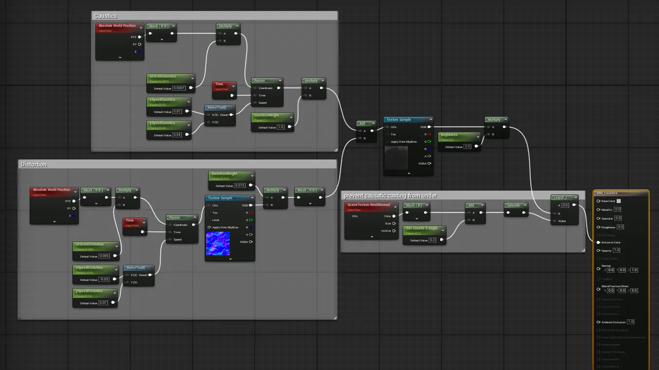
figure 24: Caustics Material
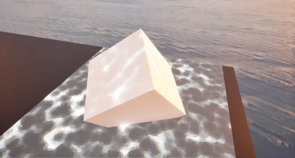
figure 25: Caustics decals
If this were to be improved upon, we can maybe project the caustics based on the sun’s position
Post-Processing, Depth, Distance fog
The post procesing effect uses distance fog based on the depth buffer to make position further away from screen become less visible. This however poses one issue, meaning that for areas above the ground, the sky, the sun will be entirely invisible.
figure 26: Opaque area above the waves
To remedy this issue, I have a few ideas
Method 1: Ray-Plane intersection against sea level
Drawing a ray plane intersection test based on sea level to see if the direction that ray points to is above the sea level or not.
To do this, world position must be reconstructed from depth. The distance from screen to the position is then compared with the distance from screen to the sea level to determine is the area above the sea is visible. For this project, I did not choose this method.
Method 2: Custom depth pass
In this method I chose to create a few objects that only draw to the custom depth pass (non-colliding, does not draw to main pass). I then set the scene and moves the mesh with custom depth to the desired sea level. This actually worked quite well lol. Although this method is not universal, this is simple and quick to setup so I opted to use this one.
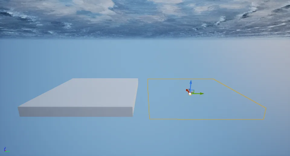
figure 27: Hiding custom depth masking object from main pass
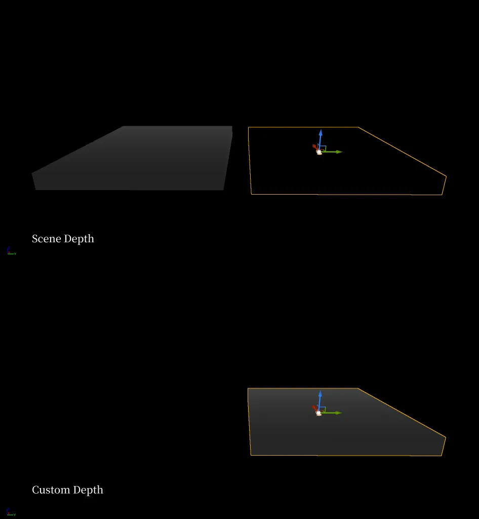
figure 28: scene vs custom depth
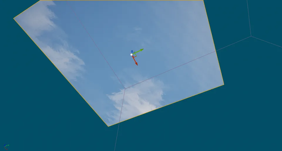
figure 29: visualizing using custom depth as mask
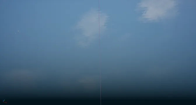
figure 30: figure26 after using custom depth
I’ve also added the sea-level based depth color which simply uses the sea-level and lerp the color based on how far one is from the sea-level. As per future improvement, if the method 1 is used, we could also get a nice gradient as well.
The final post-processing object is now done with the custom depth pass governing the scene depth based visibility and the distance form sea level governing the color.
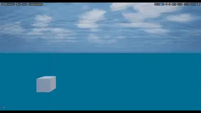
figure 31: Combining both effects
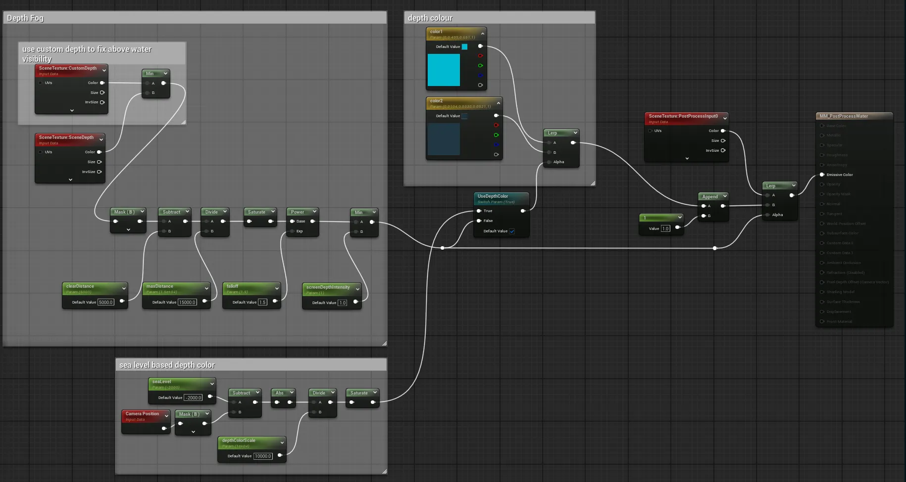
figure 32: Post-Processing material
Seagrass WPO animation - Global wind, Localwind
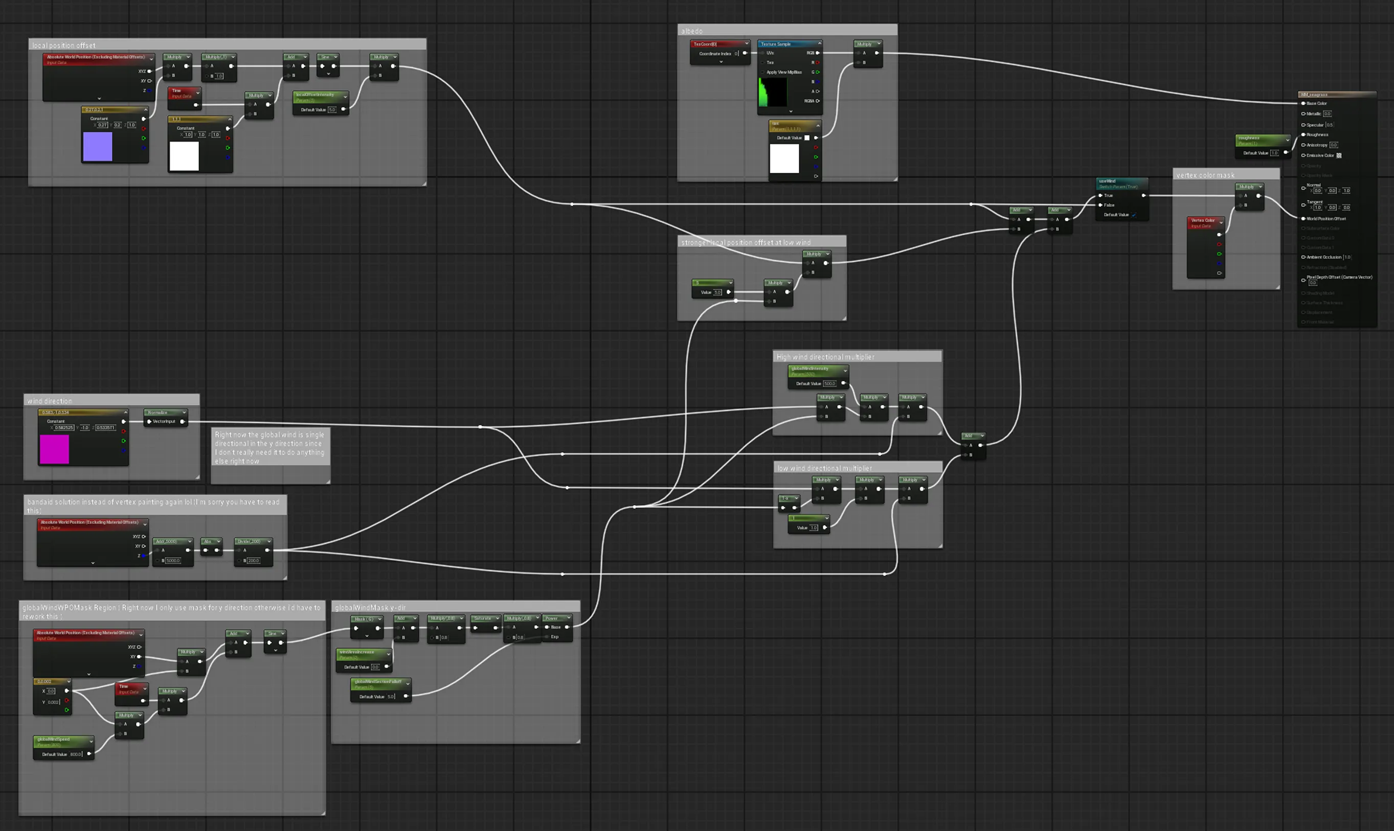
figure 33: Seagrass material
For local offset, I just use a standard wave function to offset the leaves locally.
For global wind, I just used a few normal wave funcitions for this, one to mask the position of the wind in sections. The other to move the wind, both are simple implementations of wave function.
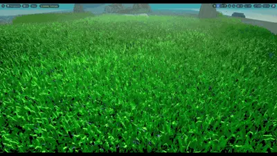
figure 34: grass wind WPO
Setting up final scenes
I first defined the camera position and since the waves, post-processing material, and caustics are already done I put them into the scene first during the grey-boxing stage.
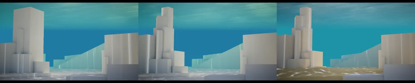
figure 35: Grey Boxing
Here I just sculpt and decimated the rock mesh and using thin cards for foliage. The materials are then later baked and exported.
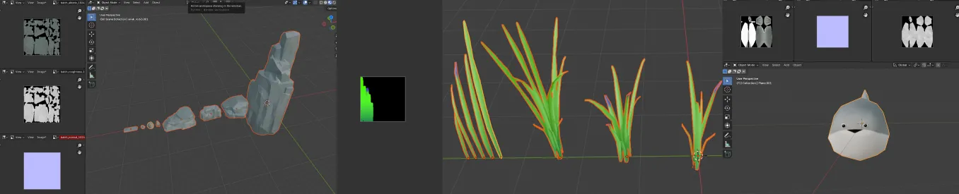
figure 36: Assets and Texture Baking
Here I swapped out blockouts, added in boids, and do some final light adjustments.
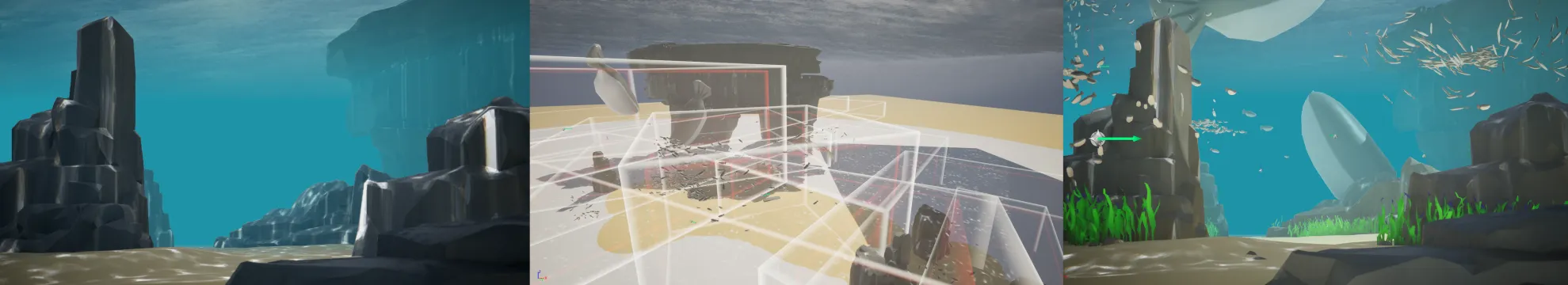
figure 37: Scene Integration
And Done!
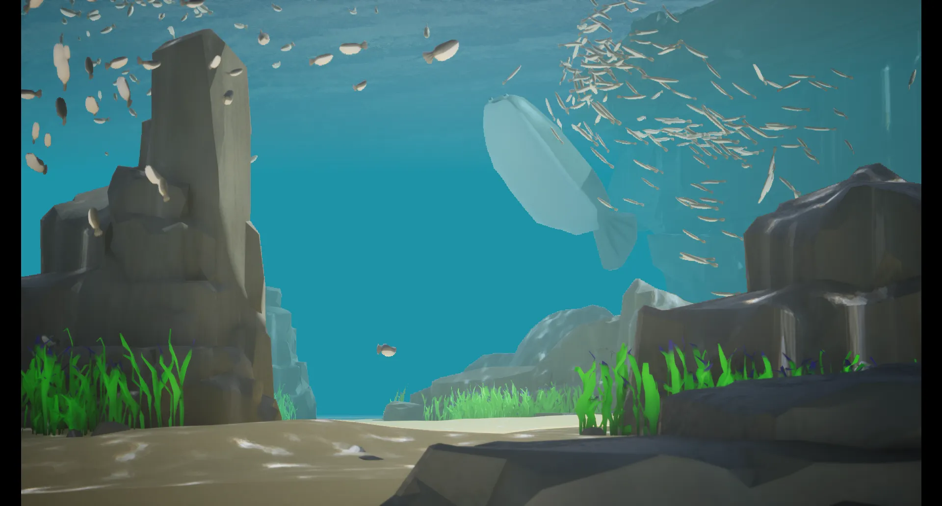
figure 38: Final Scene
References
- https://developer.nvidia.com/gpugems/gpugems/part-i-natural-effects/chapter-1-effective-water-simulation-physical-models
- https://www.youtube.com/watch?v=PH9q0HNBjT4
- https://www.youtube.com/watch?v=kGEqaX4Y4bQ
- https://cs.stanford.edu/people/eroberts/courses/soco/projects/2008-09/modeling-natural-systems/boids.html
- https://people.ece.cornell.edu/land/courses/ece4760/labs/s2021/Boids/Boids.html
- https://matthias-research.github.io/pages/tenMinutePhysics/11-hashing.pdf
- https://www.youtube.com/watch?v=82asza6Kv24
- https://www.youtube.com/@BenCloward