Abstract
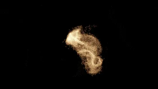
In this project, I have developed a real-time graphics engine with a high-performance particle system to simulate the movement of stars under the influence of gravitational forces. To maximizes performance, I leveraged the GPU by using compute shaders, allowing simlation up to 65,000 particles at 60+ FPS, surpassing typical CPU-based implementation which are usually limited to a few thousands particle. To enhance visual quality, I have implemented GPU instancing, allowing meshes to be rendered at each particle position. This approach allows rendering up to 10.92 million polygons (65,000 particles) with minimal performance impact. Additionally, to improve the visual fidelity, I have also implemented post-processing effects such as gaussian-blur, and bloom as well as performing HDR tone mapping and exposure controls. The engine also provides ImGui based User interface is also provided along with 2 mode cameras for user to freely interact with the scene.
※Youtube compression is not doing too well for this kind of video (preferably, try watch it from a smaller screen).
For the full source code and implementation: N-body-simulator Repository
Preface
This project is basically an educational project for me to learn how to properly use compute shaders, OpenGL, Post processing effects to make a visually stunning particle simulations. First, I must say that Physics is not my strong suit. With that given, the real aim of this project is to produce visually interesting simulation, not full physics accuracy (although I tried to be as accurate as possible). In a sense, the value in those of default test cases are extremely exaggerated so please be aware of this fact. As per the geometries of stellar clusters and how mass are mapped to colors, these are not fully accurate as well (To any physicist out there I am sorry (´;ω;`)). With that being said, the project provides multiple controllable variables for those who want to try setup the simulation for themselves as well as multiple default test cases to pick from so enjoy!! (*´ω`*)
What is an N-body simulation
The basic premises of an N-body simulation is, given an arbitrary number of particles n in a system, each and every particle in this system will interact with each other by some physical forces, which in our case is gravity. Generally this simulation is used as a tool to study dynamical system of particles, especially in fields such as astrophysics, cosmology, and molecular dynamics.
Project Scope
In this project, I have implemented a gravitational n-body variant of the simulation with the initial purpose to visually predict the motion of celestial bodies interacting with each other through gravity. The simulation is strictly gravitational using only Classical mechanics meaning there will be no collision and no insane objects like dark matter, dark energy, etc…
Implementation Methodologies
Due to the fact that currently there exist no closed-form solution for calculating the position of every particle in a dynamic system where n>2 (excluding some specific n = 3 ones). In our n-body system, we instead predict the position of each particle on the next time step based on their acceleration, velocity, and current position using something called a numerical integrator. However, in order to calculate the acceleration, we need to calculate the force of each particle which leads us to the topic of calculating force between each particle.
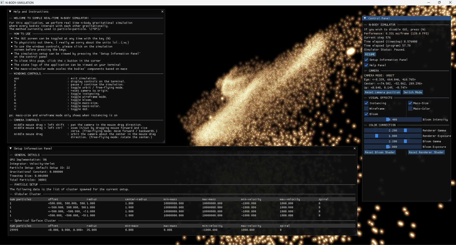
figure 0: Simulation GUI
Calculating Gravitational Force
Recall Newton’s universal law of gravitation. Let $r$ be the distance between the two particle and $m$ be the mass.
$$F= \frac{Gm_im_j}{r^2}$$
To calculate the force of one particle exerting on another ($m_j$ on $m_i$) $$F_{ij} = \frac{Gm_im_j}{||r_i-r_j||^2}\cdot -\hat{r_{ij}}$$ $$ F_{ij} = \frac{Gm_im_j}{||r_i - r_j||^2} \cdot \frac{-(r_i-r_j)}{||r_i-r_j||}$$ Using Newton’s second law of motion, we can derive the formula to calculate the acceleration of the particle using the accumulated force. $$F_{ij} = m_ia_{ij}$$ $$a_{ij} = \frac{F_{ij}}{m_i}$$ Here we can now calculate the force acting on the current particle $i$ from other particles. Let there be a particle $i$ and let $K$ be a set of particles where $|K| = n-1, i \notin K, \forall j \in K$. The acceleration of $i$ can now be calculate (accumulate) as follows. $$a_i = \sum_{j \ne i}^K a_{ij} \text{\quad;\quad} a_im_i= \sum_{j \ne i}^K F_{ij}$$ $$a_i = \frac{1}{m_i} \sum_{j \ne i}^k F_{ij} = \frac{1}{m_i} \sum_{j \ne i}^k \frac{Gm_im_j}{||r_i - r_j||^2} \cdot -\hat{r}_{ij}$$
$$= G \sum_{j \ne i}^k \frac{m_j}{||r_i - r_j||^2} \cdot -\hat{r}_{ij}$$
This can now be used to determine the acceleration of $\forall i$ in the system. Using this formula, we can calculate naively calculate acceleration of the particles using the particle-particle method, or aka. calculate all pairs. This however would be very computationally expensive having a complexity of $O(n^2)$ making the system not so scalable. In favor of performance, we could choose to opt to use methods such as Barnes-Hut or FMM that utilizes data structures such as Oct-tree to decrease the time complexity to $O(nlog(n))$ and $O(n)$ in some special case respectively. However, since I am new to compute shaders, I chose to go with the naive $O(n^2)$ method first.
Numerical Integrator
Since we now know how to calculate the acceleration, we now need to calculate the position and velocity of the particle. As for the current, there are multiple numerical integrator that can be used to address issue by approximately the velocity based on the initial information given at each timestep and proceed them based on the size of each time step.
There are multiple integrator available for physics simulation:
- Euler Integrator
- Velocity-Verlet Integrator
- RK4(Runge-Kutta 4th order)
- Hermite
- etc…
In this simulator, I’ve implemented the following two integrators:
Semi-Implicit Euler method
The idea of Euler Method is the simplest and cheapest to compute but also the most inaccurate among all aforementioned integrators due to the linearly accumulating error and inability to conserve energy. The Semi-Implicit Euler Method however conserve energy better than the standard implementation just by simply updating the velocity before position at every step (explicit version does the opposite). $$v_{i+1} = v_i + a_i * \Delta t $$ $$r_{i+1} = r_{i} + v_{i+1} * \Delta t$$
This method is a 1st order meaning:
- Local error: $O(\Delta t^2)$
- Global error: $O(\Delta t$)
Velocity-Verlet (KDK-Leapfrog)
Also known as Kick-Drift-Kick Leapfrog. This method is almost as computationally cheap as Euler, however it is a 2nd order method that also conserves energy making it more accurate. To calculate the velocity and position, simply: $$v_{i+\frac{1}{2}} = v_i + 0.5 * a_i * \Delta t$$ $$r_{i+1} = r_i + v_{i+\frac{1}{2}} * \Delta t$$ $$a_{i+1} = \text{acceleration using the new position } r_{i+1}$$ $$v_{i+1} = v_{i+\frac{1}{2}} + 0.5 * a_i * \Delta t$$
This method is a 2nd order method meaning
- Local error: $O(\Delta t^3)$
- Global error: $O(\Delta t^2)$
Engine Implementation
This project features a custom-built engine that serves as the core driver for the simulation. It is designed to model and render gravitational interactions of large clusters of celestial bodies in real-time. The engine leverages GPU acceleration through custom-written compute shaders as well as implementing techniques such as instancing and post-processing to improve the visual fidelity. The following section will explain the engine’s architecture and other important information.
Dependencies and Tools
- GLAD and GLFW for setting up and managing the OpenGL context
- GLM for mathematic operations.
- ImGui for the Graphical User Interface (GUI)
Modules
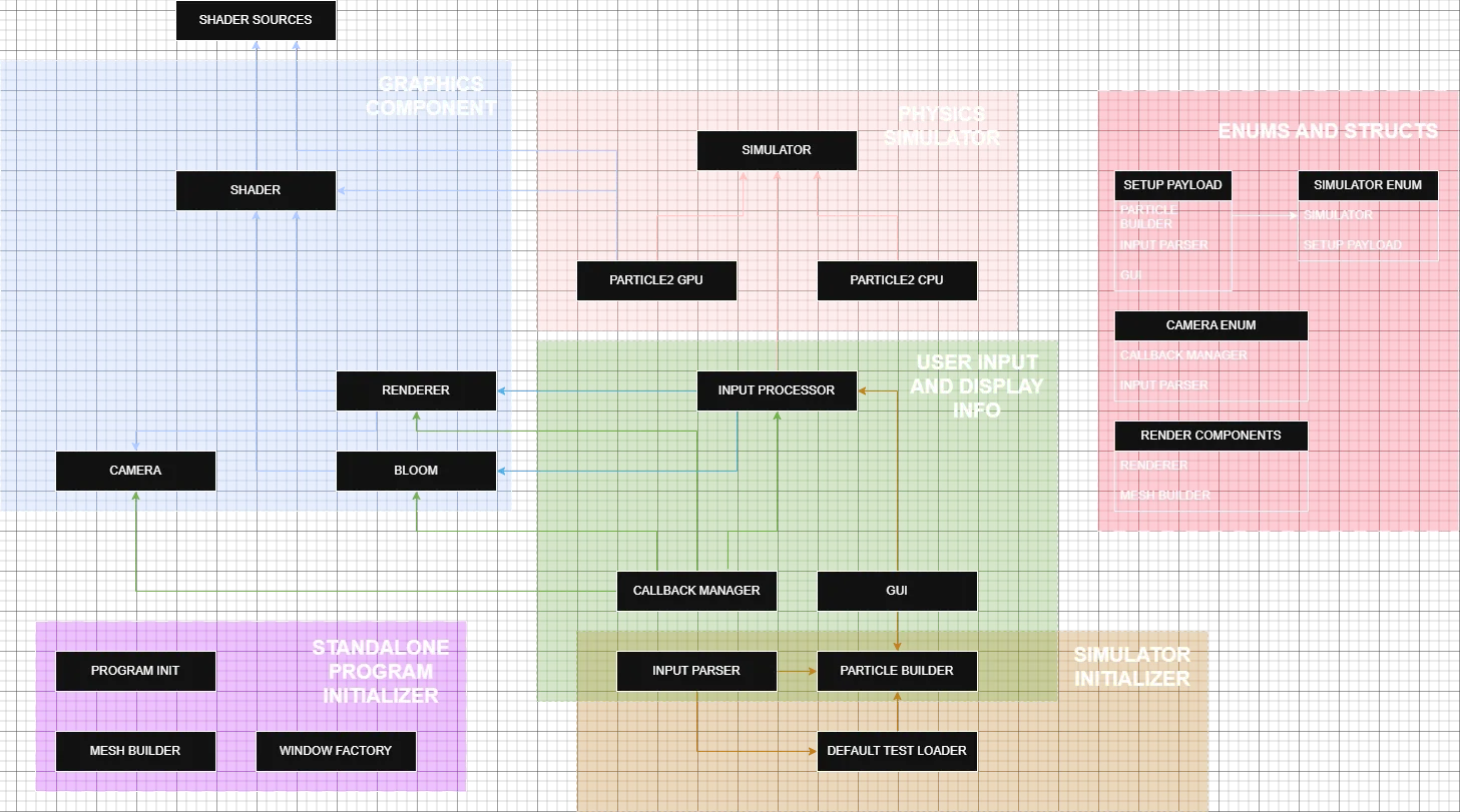
figure 1: Architecture
The modules in this engine can be grouped into 5 parts as shown in the figure above.
- The Graphics Components Modules
- Responsible for rendering frames to the window, managing mesh instancing, and applying post-processing effects such as bloom to enhance the visual fidelity of the simulation.
- The Physics Simulator Modules
- Responsible for handling the calculation of the dynamical system based on the chosen implementation and integrators.
- The User input and display information Modules
- Responsible for accepting user input from mouse control, keyboard input, and GUI toggles.
- Updates simulation and display statuses according to the user input and show the current state of the engine to the user through GUI.
- The simulation initializer Modules
- Responsible for taking in user input for initializing the particle data such as the geometry of the cluster, mass range, velocity range, number of particles for the simulator.
- The standalone program initializer Modules
- Initialize OpenGL context, creating windows, and initializing required components for sphere instancing.
- The Enums and Structs Modules
- Serves as data payload when transferring data between modules.
The Graphics and Physics Modules are designed to be independent from each other ensuring ease of modification. The User input and Display information modules however are more tightly coupled with multiple other modules due to being the interface between the users and the engine. As a result, changes in other modules would often require update in this one.
Very Brief Execution flow and Render Loop
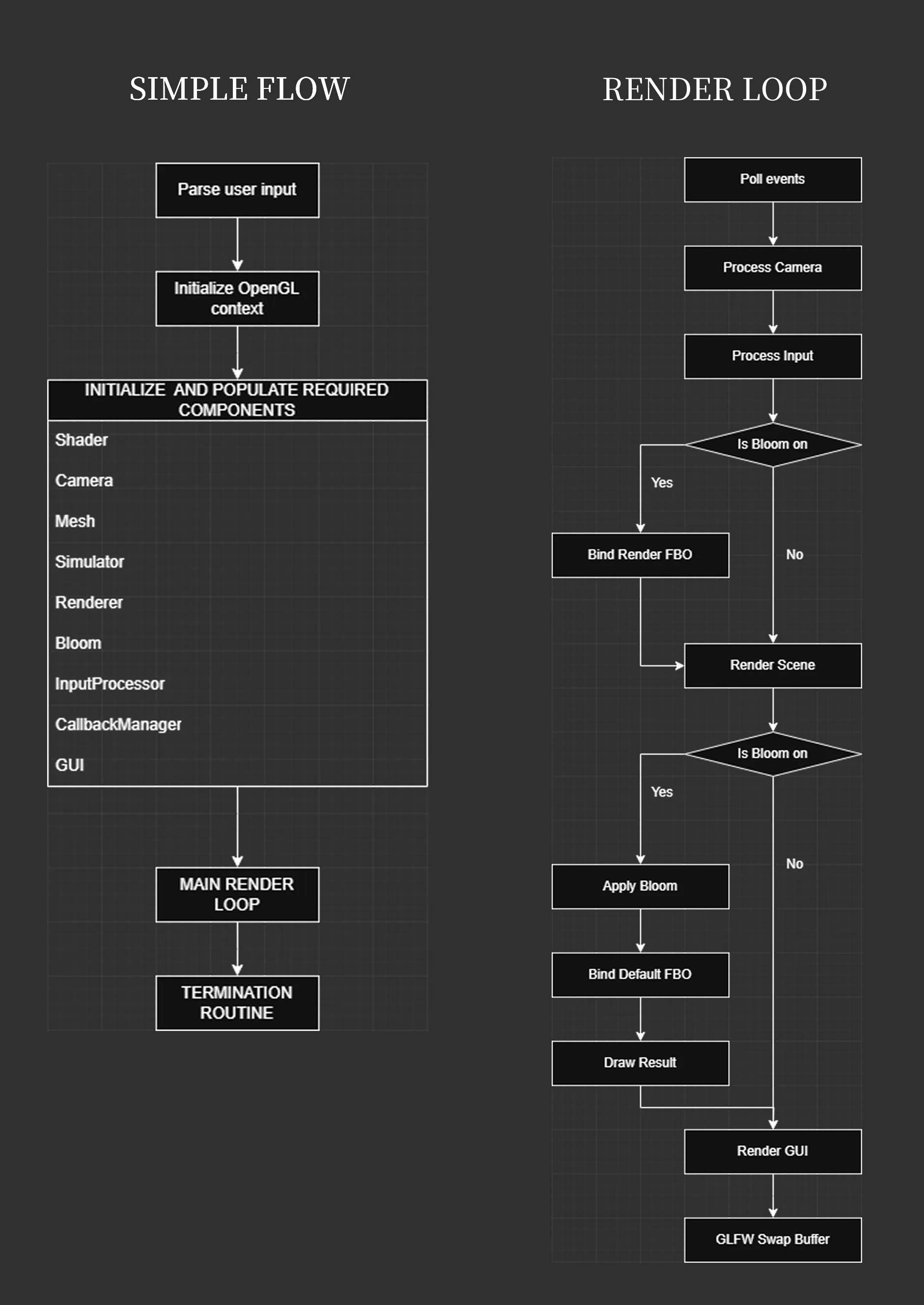
figure 2: Brief Execution Flow
Shader Pipeline and Post-Processing
The post-processing effect implemented for this engine is, for the moment just bloom and some color correction features.
Bloom
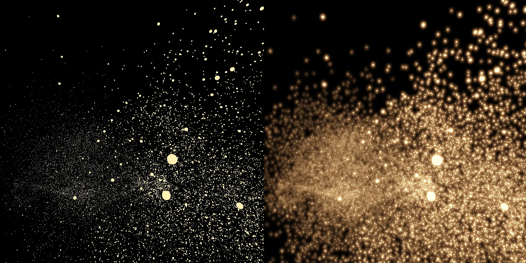
figure 3: Bloom off vs on
The idea of bloom is mostly simple. We first render the scene onto 2 separated textures. For the first texture, we keep it as the original. For the second texture, we do 2 passes gaussian blur based on the intensity we want. Afterwards we combine the two texture and do some color correction and now we have a functioning bloom output that can be used to draw on a quad.
Pipeline
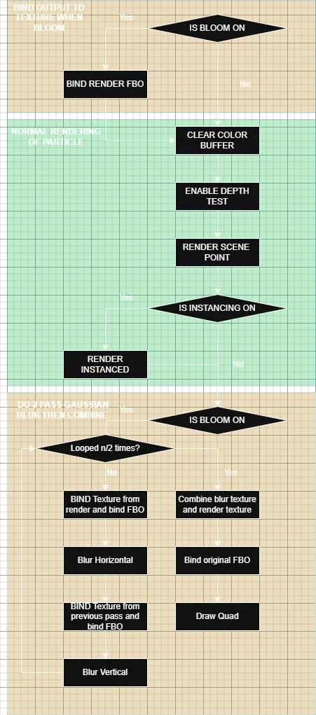
figure 4: Rendering Pipeline
In this pipeline, we can split it into 2 main paths.
- Bloom enabled:
- The main idea is basically we draw to a texture as an output, afterwards we use the texture rendered as quad for the following steps.
※ Do note that the $n/2$ in the image above is just a simplification
glFramebufferTexture2D(GL_FRAMEBUFFER, GL_COLOR_ATTACHMENT0, GL_TEXTURE_2D, tex_id, 0);
- In this case we have to bind the render of the output to bloom shader with no Color correction (tone mapping and gamma correction) to a texture.
- After that we use one of the textures to do 2 passes blur for a number of times.
- After which we combines the output with the original texture then do the color correction and renders onto a quad.
void calc_gaussian_kernel(){
    for(int i = 0; i < BLUR_RADIUS; i++){
        weight[i] = exp(-0.5*(pow(i/sigma,2)))/ (sqrt(2*3.141592653589793)*sigma) ;
    }
}

void main(){
    calc_gaussian_kernel();

    vec2 tex_offset = 1.0 / textureSize(u_prev_texture, 0); //size of texel
    vec3 color = texture(u_prev_texture, tex_coord).rgb * weight[0];

    if(is_horizontal){
        for(int i = 1; i < BLUR_RADIUS; i++){
            color += texture(u_prev_texture, tex_coord + vec2(tex_offset.x * i,0)).rgb * weight[i];
            color += texture(u_prev_texture, tex_coord - vec2(tex_offset.x * i,0)).rgb * weight[i];
        }
    } else { // vertical
        for(int i = 1; i < BLUR_RADIUS; i++){
            color += texture(u_prev_texture, tex_coord + vec2(0, tex_offset.y * i)).rgb * weight[i];
            color += texture(u_prev_texture, tex_coord - vec2(0, tex_offset.y * i)).rgb * weight[i];
        }
    }

    FragColor = vec4(color,1.0f);
}
Important Notes
- ※ Disable depth test before drawing to a quad (rectangle)
- Ensure you bind an RBO to the original scene FBO too otherwise we will some issue with depth
- Bloom disabled:
- Directly follow the path marked in green and render the scene out with color correction.
HDR, Exposure Tone Mapping and Gamma Correction
The color of the stars defined in HDR range
    vec3 yellow =vec3(5.0f, 2.0f, 0.24f);
    ...
In this case we have to perform exposure tone-mapping to allow the brightness of scene to be displayed within range of a standard screen [0,1]
color = vec3(1.0) - exp(-color * u_exposure);
Afterwards, gamma correction is then applied to ensure the color to appear correctly on standard screen.
color = pow(color, vec3(1.0/u_gamma));
Instancing
Instancing is simple, in this case we just instance all the particles as a sphere using the VAO we bind earlier and draw elements using glDrawElementsInstanced, on the Shader side, we just simply scale the vertices of the sphere by its mass then offset them by the position stored in the SSBO.
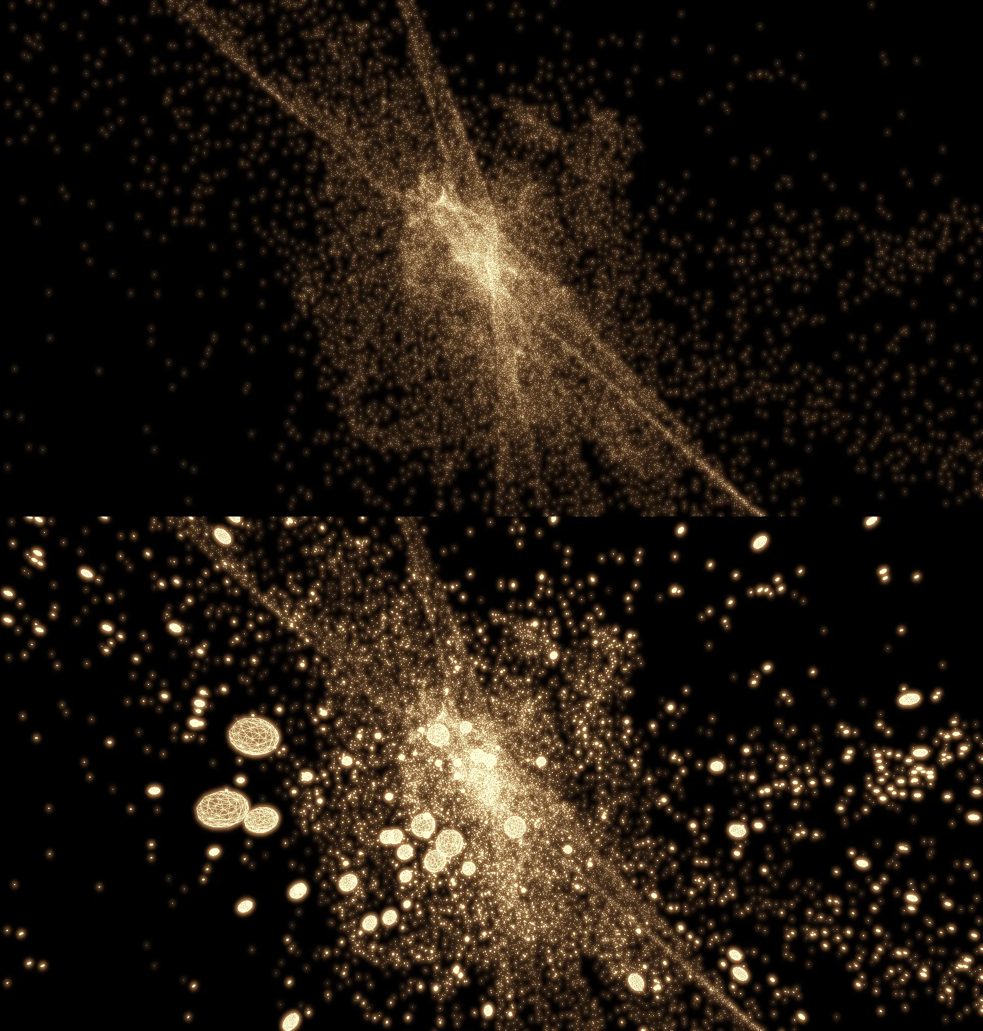
figure 5: Instancing (+Wireframe) off vs on
// CPU side
  if (!this->use_instancing)
    {
        this->shader_program->set_bool("use_instancing", this->use_instancing);
        glDrawArrays(GL_POINTS, 0, this->simulator->get_n_particle());
    }
    else
    {
        this->shader_program->set_bool("use_instancing", !this->use_instancing);
        glDrawArrays(GL_POINTS, 0, this->simulator->get_n_particle());

        this->shader_program->set_bool("use_instancing", this->use_instancing);
        glDrawElementsInstanced(GL_TRIANGLES, 3 * this->render_components->n_inds, GL_UNSIGNED_INT, (void *)0, this->simulator->get_n_particle());
    }
//light.vs
layout (std430, binding = 0) buffer particle_position {
	vec4 position[];
};
//Check the full version on my repository
...
...
...

  if(!use_instancing){
    new_pos = position[gl_VertexID];
    star_mass = mass[gl_VertexID];
  } else {
    if(use_mass_size){
      mass_size += calculate_mass_scaler(gl_InstanceID);
    }

    new_pos = position[gl_InstanceID] + vec4(mass_size * v_pos,1.0);

    star_mass = mass[gl_InstanceID];
  }
Why draw twice when instancing (specifically for our case)
Currently, we have no boundary set for our simulation meaning that once a particle moves away from the screen, it gets too tiny to get rendered onto the screen. With this issue in mind, we simply use glDrawArrays(GL_POINTS...) first to ensure that there will at least be something drawn to the screen at minimum size. Afterwards we draw the instanced version on top of the dot version. Doing this will ensure that for any area of the screen where the instanced particles are drawn, the point version will completely be blocked.
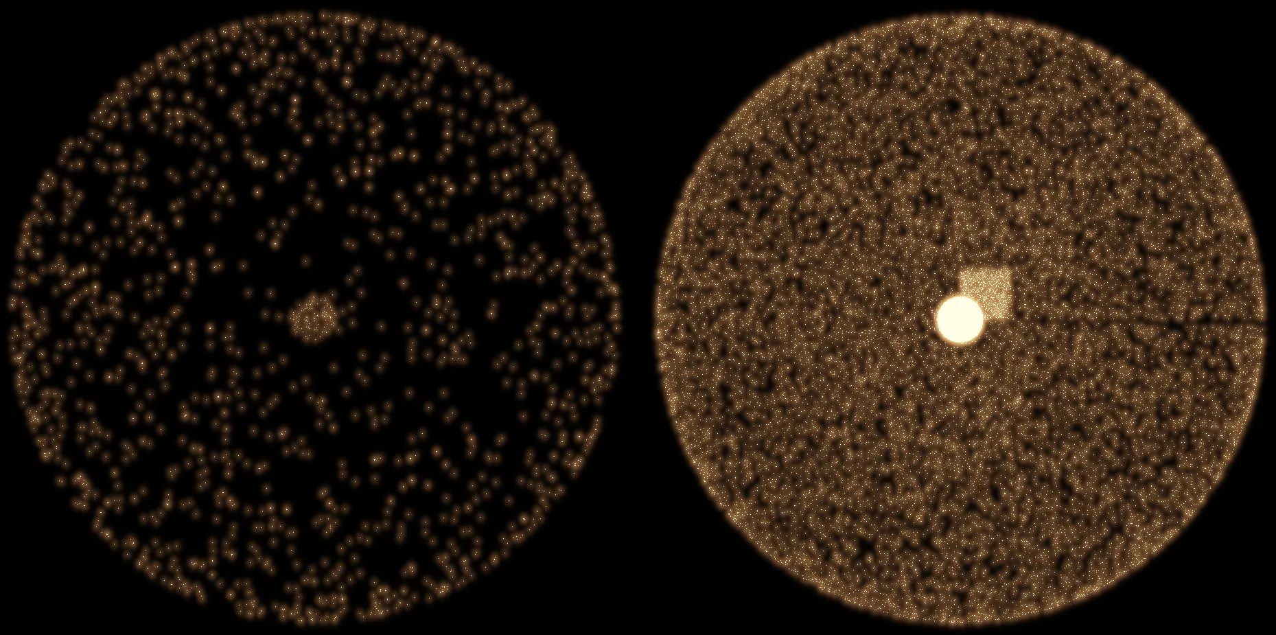
figure 6: One draw call vs double draw call
GPU optimization and performance
Performance
Due to time constraint, I have yet to make proper benchmarking scripts or setting up Nsight for performance profiling. The performance was recorded manually and averaged on the hardware this simulation was implemented in (RTX4070Ti GPU).
The FPS are written in format <Effects ON - Effects OFF>. These numbers should give a rough idea on how it should perform given this specific hardware.
| # Particles / Implementation (FPS) | CPU Naive Particle-Particle | GPU Naive Particle-Particle | GPU Tiling Particle-Particle | GPU Fine-Grain Particle-Particle |
|---|---|---|---|---|
| n = 100 | 120 | 120 | 120 | 120 |
| n = 1000 | 90-91 | 120 | 120 | 120 |
| n = 10000 | 1 | 120 | 120 | 120 |
| n = 30000 | - | 120 | 120 | 120 |
| n = 50000 | - | 88 ~ 100 | 117 ~ 120 | 109 ~ 120 |
| n = 65000 | - | 57 ~ 63 | 66 ~ 74 | 68 ~ 75 |
| n = 100000 | - | 23 ~ 23 | 37 ~ 40 | 30 ~ 32 |
| n = 150000 | - | 12 ~ 12 | 17 ~ 18 | 14 ~ 14 |
| n = 200000 | - | 7 ~ 7 | 8 ~ 8 | 8 ~ 8 |
Naive GPU Implementation
The naive implementation uses 1 workgroup per 64 particle. The idea is basically using velocity-verlet integrator to calculate the next step without further optimization.
This version does introduce some inaccuracies as well (I have yet to fix this). This is due to the fact that barrier only blocks the threads in the same workgroup, not globally, meaning that there can be some case of race conditions where position is used to calculate acceleration before some is updated.
- Work: $O(n^2)$
- Span: $O(n)$
- Available Parallelism: $O(n)$
	uint id = gl_GlobalInvocationID.x;
	if (id >= n_particle) return ;
    velocity[id] += acceleration[id] * timestep_size * 0.5;
    position[id] += velocity[id] * timestep_size;

    memoryBarrier();
    barrier();

    acceleration[id] = calculate_acceleration(id) * gravitational_constant;

    memoryBarrier();
    barrier();

    velocity[id] += acceleration[id] * timestep_size * 0.5;
Tiling - Chunk Optimized GPU Implementation
In this implementation, the idea of tiling in chunks into the shared memory has been introduced. Since fetching data repeatedly from global memory is an expensive operation. Having multiple threads in the same group collectively fetch a chunk of data into shared memory where the threads inside the same workgroup can access to calculate acceleration. This approach is likely a better approach since it reduces the amount of fetching needed to be done from global memory. This version is implemented in 2 passes.
In my case, a chunk-size of 512 and a workgroup of size x=256 seems to be the best performing settings.
const int CHUNK_SIZE = 512;
shared vec4 chunk_position[CHUNK_SIZE];
shared float chunk_mass[CHUNK_SIZE];

void main(){....
uint particle_id = gl_GlobalInvocationID.x;
uint local_id = gl_LocalInvocationID.x;
- Work: $O(n^2)$
- Span: $O(n)$
- Available Parallelism: $O(n)$
// Pre-load position of current particle if valid
    vec4 position_self = vec4(1.0f);
    if(particle_id < n_particle){
        position_self = position[particle_id];
    }

    int max_load = CHUNK_SIZE;
    uint half_chunk = 256;
    uint fetch_id = 0;

    for (uint offset = 0; offset < (n_particle + CHUNK_SIZE); offset+=CHUNK_SIZE){

        // Load chunk
        chunk_mass[local_id*2] = mass[local_id*2 + offset];
        chunk_position[local_id*2] = position[local_id*2 + offset];
        chunk_mass[local_id*2+1] = mass[local_id*2 +1 + offset];
        chunk_position[local_id*2+1] = position[local_id*2 + 1+ offset];

        memoryBarrier();
        barrier();
Here, each thread each load 2 pieces of data into shared memory per loop. From here calculation of acceleration is done as usual.
Fine-Grained GPU Implementation
In this implementation, instead of using multiple particles per workgroup. I have decided to use 1 particle per work group. However, the amount work is equally distributed among threads.
In the first pass, we use the standard 256 particle per thread implementation to update the position and velocity.
this->compute_shader_program.set_bool("first_pass", true);
glDispatchCompute(this->n_work_groups, 1, 1);
glMemoryBarrier(GL_SHADER_STORAGE_BARRIER_BIT);
this->compute_shader_program.set_bool("first_pass", false);
glDispatchCompute(this->n_particle, 1, 1);
Afterwards, for the second pass, we have shared variable setup for accumulation.
shared vec4 local_acceleration_accumulator[256];
uint particle_id = gl_WorkGroupID.x;
uint local_id = gl_LocalInvocationID.x;
The acceleration calculation is then done by having each thread accumulate the acceleration based on their local id (workgroup ID ) then add this to the shared memory before proceeding to the next stage.
    for (uint i = local_id; i < uint(n_particle); i+= 256){
        tmp_distance = position[particle_id] - position[i];
        if(tmp_distance != vec4(0.0)){
            tmp_direction = -normalize(tmp_distance);
            sq_distance = dot(tmp_distance,tmp_distance);
            local_acceleration_sum += (mass[i]/sqrt(sq_distance+sq_soften)) * tmp_direction;
        }
    }

    local_acceleration_accumulator[local_id] = local_acceleration_sum;
    barrier();
After accumulating all the acceleration locally, we then accumulate the acceleration using tree based reduction until acceleration at local_id 0 have the sum of all acceleration.
    for (uint stride = 128; stride > 0; stride >>=1) {
        if(local_id < stride){
            local_acceleration_accumulator[local_id] += local_acceleration_accumulator[local_id + stride];
        }
        barrier();
    }
Afterwards we calculate the velocity as usual.
- Work: $O(n^2)$
- Span: $O(n)$
- Available Parallelism: $O(n)$
2 Passes and Global Synchronization
Since the order of computation of velocity-verlet is
- Calculate half velocity
- Calculate new position
- Calculate acceleration
- Calculate half velocity
Between step 2 and 3, if some workgroup finishes faster than the other, we might have issue where the acceleration is calculated using the position other variables of the previous step creating minor accuracies that accumulate overtime.
To counter this issue, one way is to use 2 compute dispatch separated by global memory barrier.
        this->compute_shader_program.set_bool("first_pass", true);
        glDispatchCompute(this->n_work_groups, 1, 1);
        glMemoryBarrier(GL_SHADER_STORAGE_BARRIER_BIT);
        this->compute_shader_program.set_bool("first_pass", false);
        glDispatchCompute(this->n_work_groups, 1, 1);
something like this, to ensure that the value syncs before we update the next step.
Future Improvements
- Further optimization on the particle interaction calculations (use oct-tree, FMM, Barnes-Hut…)
- More effects?
- Save-Load system
Known Issues
- If you set the velocity or mass to some crazy stuffs and you start to see some void ball in the middle of your screen, fear not for the stuffs is actually flying off the camera limit… 😂 [Will need to set world boundary probably]
- The sphere is sampled using
glm::sphericalRandso there is a gaping hole and a line on some position… - Particle-Particle NAIVE GPU have very minor inaccuracy issue due to being done in 1 pass
References and Resources
Here are list of resources I read while researching on how to build this simulator, you will probably find them useful if you want to dive deeper into this subject!
- https://learnopengl.com/
- https://www.youtube.com/@OnurMutluLectures
- https://en.wikipedia.org/wiki/n-body problem. (n.d.).
- https://en.wikipedia.org/wiki/Leapfrog_integration
- Dehnen, W., & Read, J. (2011). N-body simulations of gravitational dynamics. arxiv:1105.1082v1.
- Brandt, A. (2022, 03). On distributed gravitational n-body simulations, arxiv:2203.08966. https://arxiv.org/pdf/2203.08966
- Computation and astrophysics of the n-body problem. (n.d.). Graps, A. (1996). N-body / particle simulation methods. https://www.cs.cmu.edu/afs/cs/academic/class/15850c-s96/www/nbody.html
- https://www.algorithm-archive.org/contents/verlet_integration/verlet_integration.html
- https://developer.nvidia.com/gpugems/gpugems/part-vi-beyond-triangles/chapter-37-toolkit-computation-gpus
- https://developer.nvidia.com/gpugems/gpugems3/part-v-physics-simulation/chapter-31-fast-n-body-simulation-cuda